Applications in Root Cause Analysis : BPI

Overview

In this experiment, we demonstrate an application of partial ranking in Business Process Intelligence.

A business process can be viewed as a sequence of tasks that need to be performed to achieve a specific business objective. In large organizations, such processes are typically complex and hard to optimize, and enterprise tools are often used to monitor and improve such processes (an overview of such tools can be found in this link). We now show how partial ranking methodologies can be helpful in improving the insights provided by such tools.

The Data

Let us consider the Purchase-to-Pay (P2P) business process, which involves the activities encountered while acquiring goods or services from external suppliers. For every purchase request, the sequence in which the activities are executed is captured by sophisticated Enterprise Resource Management systems like SAP. A particular sequence of activities is referred to as a process variant, and in large organizations, there are typically hundreds of process variants for a business process like P2P. We consider a P2P dataset from an SAP system of certain organization provided by a German data processing company - Celonis, during a hackathon event organized in collaboration with RWTH Aachen University in April 2022.

Access to the data:

The SAP P2P Hackathon 2022 dataset can be requested for access through Celonis Academy. Once this dataset is available to you through the cloud service of Celonis, it can be downloaded by running the script examples/get_data_from_celonis.py after entering your credentials. Then, the CSV files examples/data/sap_p2p_events.csv and examples/data/sap_p2p_cases.csv would become available.

import pandas as pd

df_events = pd.read_csv('data/sap_p2p_events.csv',sep=',')
df_events = df_events.drop(columns=['Unnamed: 0'])

df_case = pd.read_csv('data/sap_p2p_cases.csv',sep=',')
df_case = df_case.drop(columns=['Unnamed: 0'])

Understanding the data:

Every purchase request or case is uniquely identified by an ID indicated in the column case:concept:name. In sap_p2p_cases.csv, there is a record for each purchase request, which is associated with a specific sequence of activities or events (case:variant). The duration of every request in seconds is indicated in the column timestamp.

df_case.head()

	case:concept:name	case:variant	duration
0	800000000047700009	Create Purchase Requisition Item, Create Purch...	41760.0
1	800000000088700005	Create Purchase Requisition Item, Create Purch...	38880.0
2	800000000129700001	Create Purchase Requisition Item, Create Purch...	43200.0
3	800000000170600007	Create Purchase Order Item, Print and Send Pur...	28800.0
4	800000000211600003	Create Purchase Requisition Item, Create Purch...	53280.0

Multiple cases can be mapped to a particular variant. The number of cases and the number of unique variants are shown below:

num_cases = df_case['case:concept:name'].unique().shape[0]
num_variants = df_case['case:variant'].unique().shape[0]

print(f'Number of cases: {num_cases}')
print(f'Number of variants: {num_variants}')

Number of cases: 279020
Number of variants: 562

Each variant is assigned a unique ID. We then identify the variants that were observed in more than 100 cases, and prepare the durations data in the following format:

durations = {
    0: [42032,76321,...],
    1: [65434, 23432, ...],
    ...
}

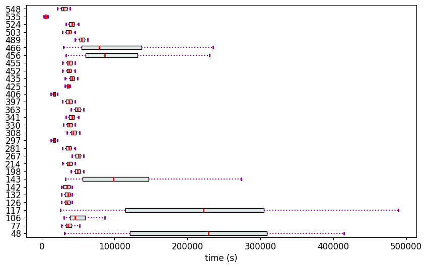
The data is then visualized.

from partial_ranker import MeasurementsVisualizer

df_case['variant_id'] = df_case.groupby(['case:variant']).ngroup()
var_id_dict = dict(zip(df_case['case:variant'], df_case['variant_id']))
ranking_inp = dict(df_case.groupby('variant_id')['duration'].apply(list))

durations = {}
for k,v in ranking_inp.items():
    if len(v)>100:
        durations[str(k)] = v

mv = MeasurementsVisualizer(durations)
fig = mv.show_measurements_boxplots(scale=0.2)

In the other file sap_p2p_events.csv, there is a record for every event along with its associated timestamp. This data is rather redudant for our experiment, but will be required by the library pm4py that calculates the Directly Follows Graph later on.

df_events.head()

	case:concept:name	concept:name	case:variant	timestamp
0	800000000006800001	Create Purchase Requisition Item	Create Purchase Requisition Item, Create Purch...	2008-12-31 07:44:05
1	800000000006800001	Create Purchase Order Item	Create Purchase Requisition Item, Create Purch...	2009-01-02 07:44:05
2	800000000006800001	Print and Send Purchase Order	Create Purchase Requisition Item, Create Purch...	2009-01-05 07:44:05
3	800000000006800001	Receive Goods	Create Purchase Requisition Item, Create Purch...	2009-01-12 07:44:05
4	800000000006800001	Scan Invoice	Create Purchase Requisition Item, Create Purch...	2009-01-20 07:44:05

Partial Ranking of the Variants

We first apply Methodology 2 (partial_ranker.PartialRankerDFGReduced) to rank the variants.

from partial_ranker import QuantileComparer
from partial_ranker import PartialRankerDFGReduced

comparer = QuantileComparer(durations)
comparer.compute_quantiles(q_max=75, q_min=25,outliers=False)
comparer.compare()
pr_dfg_r = PartialRankerDFGReduced(comparer)
pr_dfg_r.compute_ranks()

h0 = pr_dfg_r.graph_H.get_separable_arrangement()

print("Reordering and visualizing the data again")
mv = MeasurementsVisualizer(durations, h0)
fig = mv.show_measurements_boxplots(scale=0.2)

Reordering and visualizing the data again

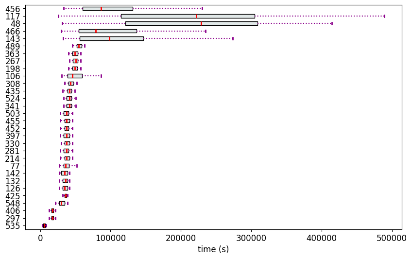
The Ranks (Methodology 2)

We see that except the variants 535,297 and 406, all the other variants collapse into a single rank. This is not ideal to discriminate the variants. Therefore, we recalculate the ranks using Methodology 1 (partial_ranker.PartialRankerDFG).

R = pr_dfg_r.get_ranks()
for k,v in R.items():
    print(f'Rank {k}: {v}')

Rank 0: ['535']
Rank 1: ['297', '406']
Rank 2: ['548', '425', '126', '132', '142', '77', '214', '281', '330', '397', '452', '455', '503', '341', '524', '435', '308', '106', '198', '267', '363', '489', '143', '466', '48', '117', '456']

The Ranks (Methodology 1)

from partial_ranker import PartialRankerDFG

pr_dfg = PartialRankerDFG(comparer)
pr_dfg.compute_ranks()

R = pr_dfg.get_ranks()
for k,v in R.items():
    print(f'Rank {k}: {v}')

Rank 5: ['48', '117', '143', '456', '466']
Rank 2: ['77', '126', '132', '142', '214', '281', '330', '397', '425', '452', '455', '503', '548']
Rank 3: ['106', '308', '341', '435', '524']
Rank 4: ['198', '267', '363', '489']
Rank 1: ['297', '406']
Rank 0: ['535']

Now the variants are classified into more ranks. The rank dependency graph is shown below:

pr_dfg.get_dfg().visualize()

Mining for the Causes of Performance Differences

1. Creating a best/worse bifurcation of the ranks: We do not find a nice bifurcation as in the GLS example.Therefore, based on a visual inspection of the DFG and box plots, we decided to mine for performance differences between the variants in \(good = \{Rank 0, Rank 1, Rank 2\}\) and \(bad = \{Rank 5\}\). Note that the BPI tools allow for interactive analysis based on visual inspection.

2. Identify the dependencies among the events: We use the pm4py library to prepare a Directly-Follows Graph (DFG); there is a node for every unique event and an an edge from eventA to eventB exists if eventA immediately follows eventB in atleast one of the cases.

3. Graph coloring: We color the nodes and edges of the graph as follows:

• The nodes and edges that occur only in the \(good\) variants are indicated in green.

• The nodes and edges that occur only in the \(bad\) variants are indicated in red.

• The nodes and edges that occur both in both \(good\) and \(bad\) are not colored.

good = R[0]+R[1]+R[2]
bad = R[5]

good = list(map(int, good))
bad = list(map(int, bad))

from pm4py.objects.conversion.log import converter as log_converter
from variants_compare import VariantsCompare

df_events['case:variant_id'] = df_events.apply(lambda x: var_id_dict[x['case:variant']], axis=1)
df_ = df_events.drop(columns=['case:variant'])
xes_log = log_converter.apply(df_)

vc = VariantsCompare(xes_log, good, bad, variants_id_key='variant_id')
gviz = vc.get_dfg_minus_best_worst()
gviz