Usage

The required input to use this library is a set of objects, each with a set of scalar values, represented as a dictionary. For the purpose of demonstration, we simulate the measurement values by sampling from normal distribution. To this end, the module MeasurementsSimulator can be used. In the following example, we create 4 objects with measurements simulated from two normal distributions differing in mean and standard deviation.

from partial_ranker import MeasurementsSimulator

#Normal distribution 1
n1 = [0.3,0.01] # [mean1, std1]

#Normal distribution 2
n2 = [0.35,0.01] # [mean2, std2]

M = {}
M['t0']  = n1
M['t1']  = n1
M['t2']  = n1
M['t3']  = n2

ms = MeasurementsSimulator(M,seed=3)
ms.measure(reps=5)
measurements = ms.get_measurements()

for m,v in measurements.items():
    print(f'{m}:{v}')

t0:[0.3178862847343032, 0.3043650985051199, 0.3009649746807201, 0.2813650729663551, 0.297226117974856]
t1:[0.2964524102073101, 0.29917258518517537, 0.2937299932317615, 0.2995618183102407, 0.29522781969640494]
t2:[0.2868613524663732, 0.3088462238049958, 0.3088131804220753, 0.31709573063652946, 0.3005003364217686]
t3:[0.3459532258539911, 0.3445464005238047, 0.3345352268441703, 0.35982367434258156, 0.33898932369888524]

Visualizing the Measurements

The set of measurements for each object can be visualized as a box-plot using the module MeasurementsVisualizer.

from partial_ranker import MeasurementsVisualizer
mv = MeasurementsVisualizer(measurements)
fig = mv.show_measurements_boxplots(scale=0.5)

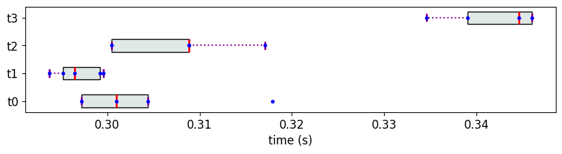
The box represents the Inter Quartlie Interval (IQI), which is the interval between the 25th and the 75th quantile values, and the red line with the box represents the median value.

The Comparison Matrix

The comparison matrix (C) is a square matrix of size \((N \times N)\), where \(N\) is the number of objects. This matrix holds the results of pair-wise comparisons among the objects as follows:

• If t_i is better than t_j, then C[t_i][t_j] = 0.

• If t_i is equivalent to t_j, then C[t_i][t_j] = 1.

• If t_i is worse than t_j, then C[t_i][t_j] = 2.

The module QuantileComparer implements the better-than relation by comparing the IOIs; t_i is considered to be better than t_j if and only if the IOI of t_i lies entirely to the left of the IOI of t_j. If the IQI of t_i and t_j overlap with one another, then t_i and t_j are considered equivalent or incomparable.

The comparison matrix for the samples of measurements is shown below:

from partial_ranker import QuantileComparer
import pandas as pd

cm = QuantileComparer(measurements)
cm.compute_quantiles(q_max=75, q_min=25)
cm.compare()
pd.DataFrame(cm.get_comparison_matrix())

	t0	t1	t2	t3
t0	-1	1	1	2
t1	1	-1	2	2
t2	1	0	-1	2
t3	0	0	0	-1

Partial Ranking of the Objects

The module PartialRanker takes as input the object holding the comparison matrix, in our case - QuantileComparer, and assigns a partial rank to the objects.

from partial_ranker import PartialRanker

pr = PartialRanker(cm)
pr.compute_ranks()

R = pr.get_ranks()
for k,v in R.items():
    print(f'Rank {k}: {v}')

Rank 0: ['t1', 't0', 't2']
Rank 1: ['t3']

Notice that the objects t0, t1 and t2, which were sampled from the same distribution, are grouped in the same rank despite the IQI of t1 and t2 not overlapping with one another. As mentioned earlier, non-transitivity of the better-than relation leads to more than one reasonable partial rankings, and it is also possible to not have t1 and t2 in the same rank. This can be achieved by changing the methodology of the parital ranking.

At the moment, three different methodologies for partial ranking described in the paper are implemented in this library. They are:

• PartialRankerDFG (Methodology 1)

• PartialRankerDFGReduced (Methodology 2)

• PartialRankerMin (Methodology 3)

If the methodology is not explicitly specified, PartialRankerDFGReduced would be used.

Partial ranks according to PartialRankerDFG:

from partial_ranker import Method

pr.compute_ranks(Method.DFG)

R = pr.get_ranks()
for k,v in R.items():
    print(f'Rank {k}: {v}')

Rank 0: ['t0', 't1']
Rank 1: ['t2']
Rank 2: ['t3']

Partial ranks according to PartialRankerMin:

pr.compute_ranks(Method.Min)

R = pr.get_ranks()
for k,v in R.items():
    print(f'Rank {k}: {v}')

Rank 0: {'t1', 't0', 't2'}
Rank 1: {'t3'}

In the following section, the behaviour of the different methodologies are demonstrated. In a later section, a couple of experiments to demonstrate the applications of partial ranking have been documented.